The Influence of Handlebar Geometry on Torsional Stability and Controllability of Road Racing Bicycles: A Dynamic Systems Analysis
1. Introduction: the handlebar as primary interface for control and stability
1.1. Context of bicycle stability
Bicycle stability is a complex phenomenon resulting from delicate interaction of multiple physical factors. Traditional understanding of bicycle dynamics is founded on a triad of stabilizing mechanisms: the gyroscopic effect generated by rotating wheels, the caster effect produced by positive mechanical trail, and mass distribution within the system. While these principles are intrinsic to bicycle design, their effectiveness is profoundly modulated by rider-machine interaction. This interaction occurs primarily through the handlebar, which serves as the primary interface for control and stabilization.
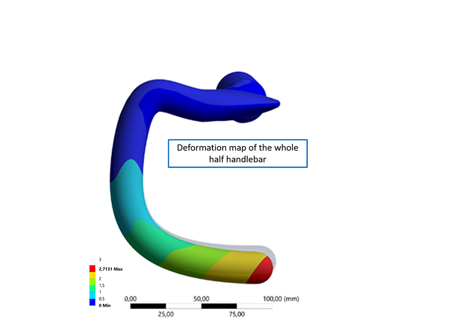
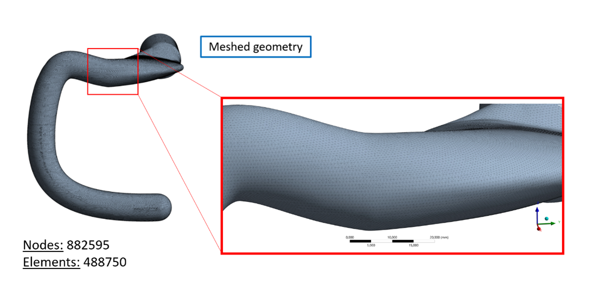
The study was developed matching
– Digital dynamic simulations from 3D models
– Accellerometer data in real conditions
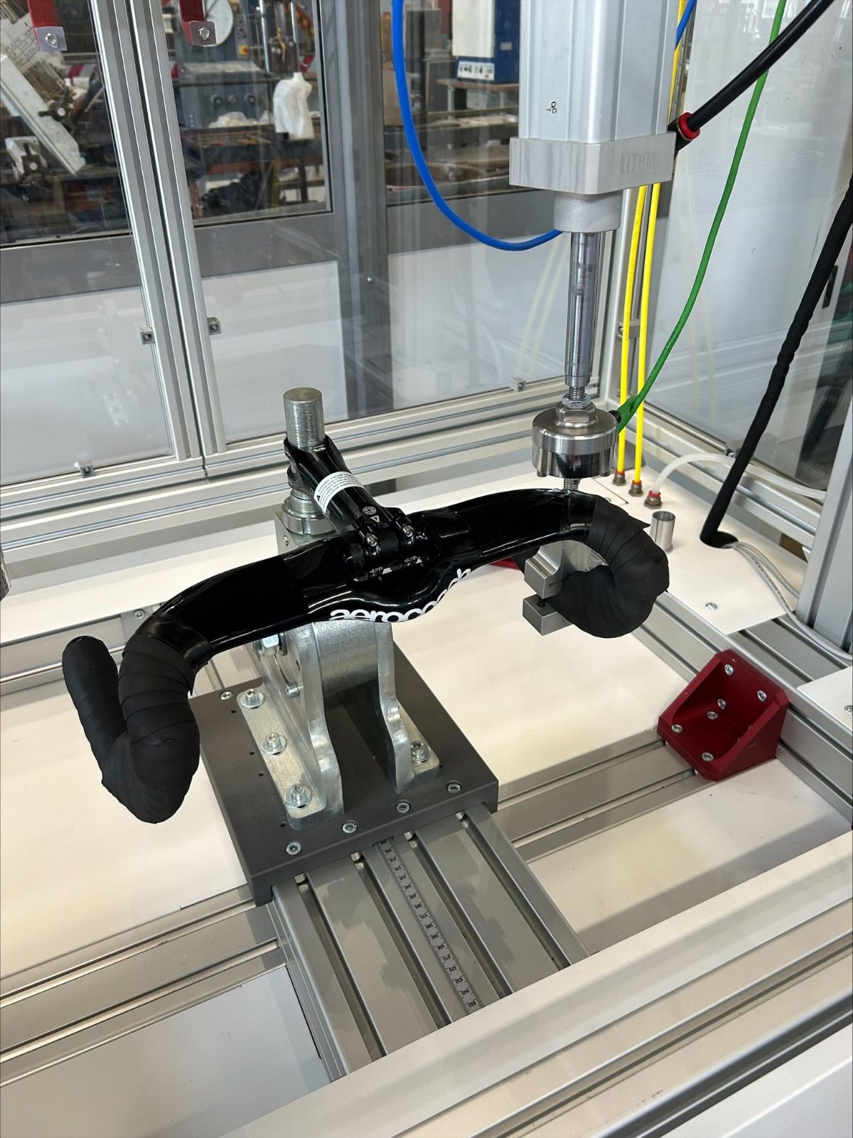
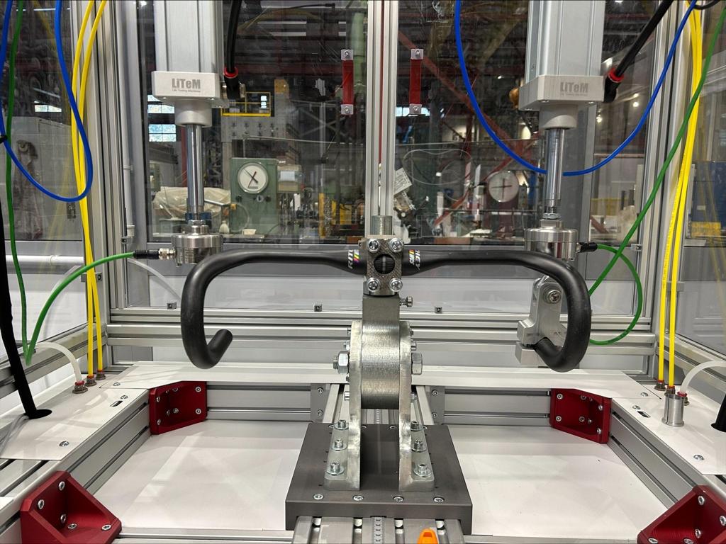
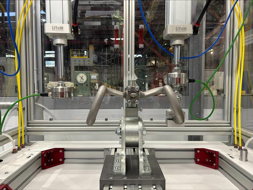
– Laboratory test with customized testing machines

1.2. The multifactorial role of the handlebar
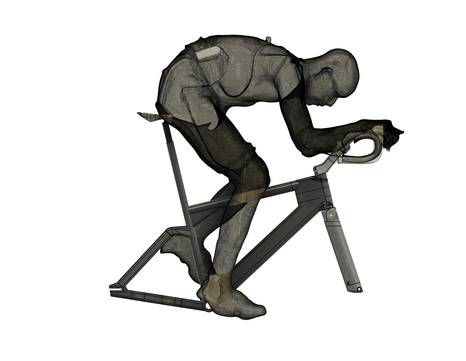
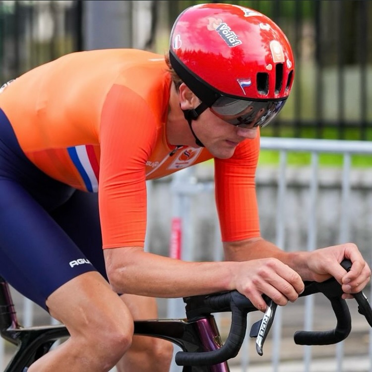
The handlebar transcends its function as a simple ergonomic component. It is the interface for direct steering input, but more critically, its geometry (width, reach, and height) determines the upper body posture of the rider. This posture directly influences the position of the combined Center of Mass (CoM) of the rider-bicycle system. CoM modulation is the central mechanism through which handlebar geometry affects overall vehicle dynamics, a fundamental concept that will be developed in this study.
1.3. Problem definition: the “shimmy” phenomenon
The specific instability investigated in this study is the high-frequency torsional oscillation of the front end, commonly known as “shimmy” or “speed wobble”. This phenomenon is described as a self-excited vibration emerging from resonant coupling of natural frequencies of system components (frame, fork, wheels). The study investigates how handlebar geometry can be optimized to increase system resistance to such instabilities, thereby improving rider safety and confidence at high speeds.
1.4. Research objectives and hypothesis
Primary Objective: Develop and validate a theoretical model linking handlebar geometric parameters (W, R, S) to quantifiable dynamic stability metrics (oscillation amplitude, damping time).
Secondary Objective: Propose and physically interpret a new composite metric, the Stability and Agility Factor (StabFactor), defined as (RxS)/(W/2) as a predictor of both passive stability and active controllability.
Hypothesis: The study hypothesizes that a higher value of StabFactor is directly correlated with greater torsional stability and faster oscillation damping velocity.
The conventional view often presents a compromise between stability (associated with long wheelbase or slack head angle) and agility (associated with short wheelbase or steep head angle). This study reframes the discussion, proposing that specific handlebar geometries can simultaneously improve both passive stability and a specific form of high-speed agility known as “lean steering”. The analysis therefore extends beyond investigating stability to optimizing the human-machine control loop under dynamic riding conditions.
1.5 Beyond the Static Lever: The Failure of the 2D Model
Traditional analysis of cockpit stability, and consequently the regulations that govern it (e.g., UCI rules ), makes a fundamental error: it treats the handlebar as a two-dimensional, static “steering wheel.
It’s not a matter of “mountain bike” equilibrism and “superlow spees” cornering where the effective rotation of the wheel caosed by the handlebar rotation around his axle prodice the cornering effect.
In the road bike
This “static” (or low-speed) model presumes that control is achieved by applying a symmetric torsional torque \(\tau_S\) to “steer,” as if one were using a balancing rod to manage a slow-moving mass. In this flawed model, a greater width (W), which provides a longer lever, is illogically considered a “safety” feature.
The reality of high-speed riding is governed by a completely different model: a three-dimensional kinematic model.
At high speed, “if you turn the handlebars, you fall.”
Control is no longer static.
The dynamic kinematics of motion require that a corner is the result of balancing centripetal and centrifugal forces, initiated by a split-second of counter-steering (“pulling”) or by a shift in the center of mass (“lean steering”).
In this dynamic model, the true control levers are not W, but the system’s ability to self-stabilize (Passive Stability) and the rider’s ability to manage the bike’s inclination (Active Control). We must therefore abandon the 2D analysis and define stability in its true three-dimensional context.
1.6 A Note on the “Mountain Bike Fallacy” and Static vs. Dynamic Control
A common objection, and a primary source of industry misconception, is the observation: “But mountain bikes use wide handlebars for stability.” This argument is a fallacy, as it fundamentally confuses two different domains of physics and vehicle control.
It’s not a matter of “mountain bike” equilibrism and “super-low speed” cornering where the effective rotation of the wheel, caused by the handlebar rotation around its axle, produces the cornering effect. That model relies on the handlebar (W) as a static “balancing rod,” where a wider lever provides more authority to manage a mass at low velocity.
This analogy of the balancing rod completely collapses at high speed.
The idea of a balancing rod being easier to manage is only true without speed. Imagine trying to run on a balance beam while holding a large, wide balancing rod.
The rod’s own inertia and its susceptibility to external forces would make you less stable, not more. This is the correct model for high-speed cycling. The wide lever (W) becomes a liability that amplifies external perturbations \(\tau_I\), rather than an asset for control.
The objection of the “long lever” (the wide MTB bar) being more stable is the effect of a common misconception (un luogo comune), not the reality of the data.
This study, and its simplified 1-DOF model, analyzes the dynamic, non-elementary kinematic behavior of a high-speed system. This is precisely why the StabFactor model—which proves that stability is driven by the 3D relationship \(R \times S\) while being penalized by W—is correct.
1.7 The 3D Origin of Stability: From Trigonometry to the StabFactor
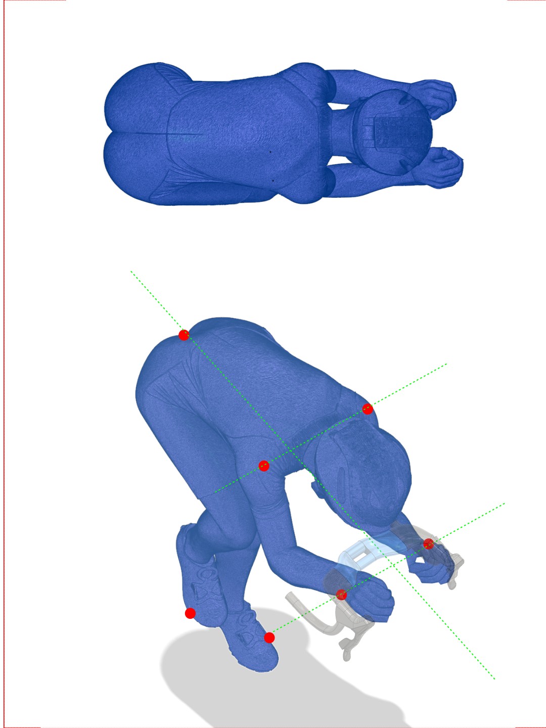
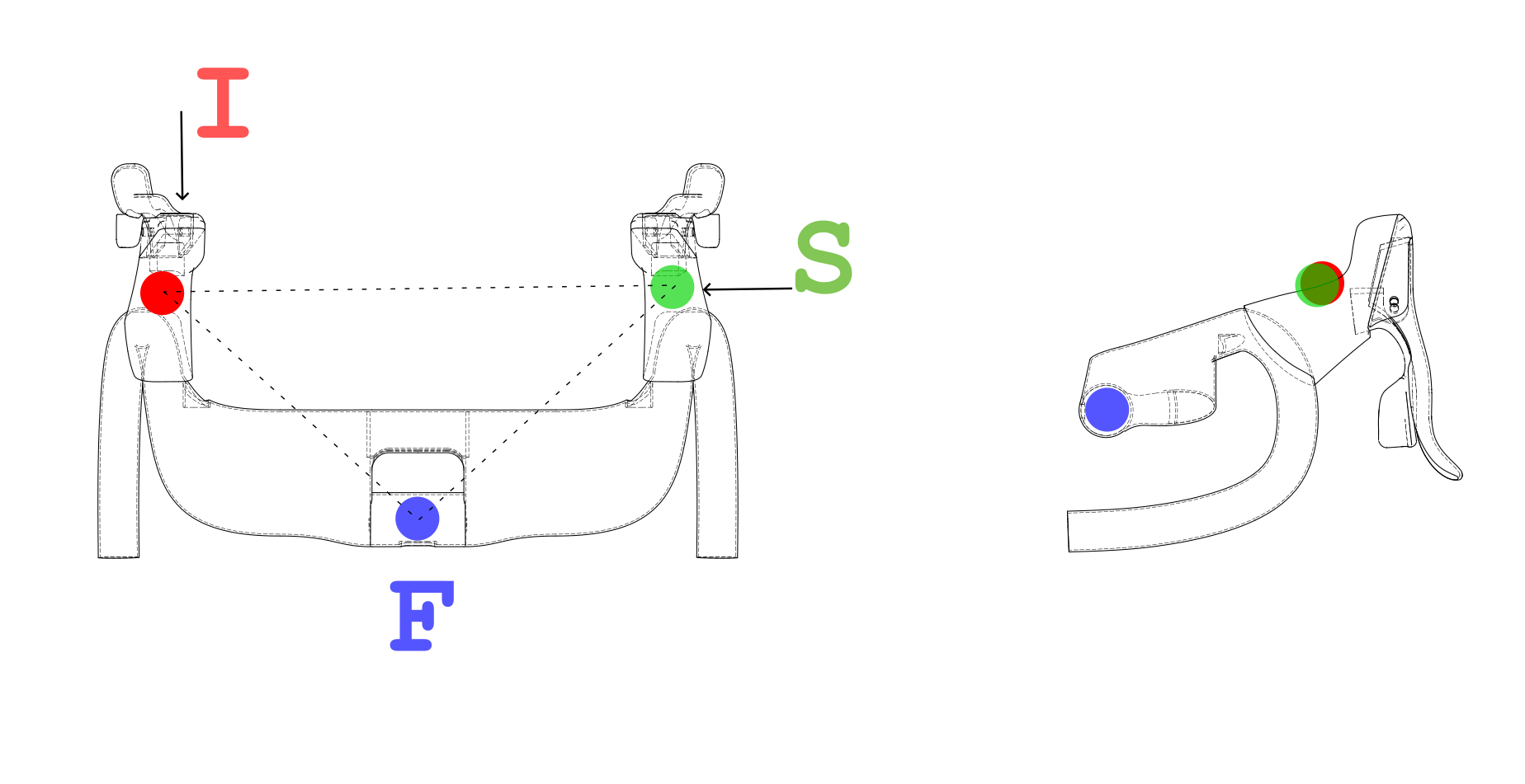
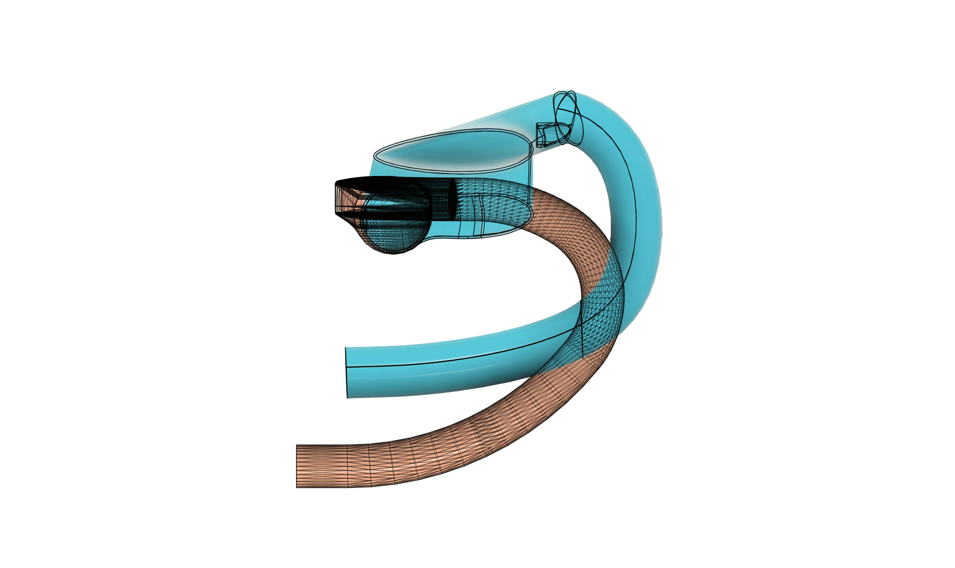
If the 2D model is fallacious, stability must originate from the cockpit’s true 3D geometry, with the steering fulcrum (the Blue Point) as the origin. The true control parameters become the 3D coordinates of the hand support points (Red and Green Points):
- Reach (R or X-Axis): The longitudinal lever.
- Stack (S or Z-Axis): The vertical lever.
- Width (W/2 or Y-Axis): The lateral lever.
Our study experimentally revealed (through dynamic testing with accelerometers, as explained in the Methodological Note) that stability is dominated by the product of \(R \times S\). This relationship is not arbitrary; it is the simplification of a fundamental trigonometric proof.
1.8 The Trigonometric Proof
Let us analyze the system in the X-Z plane (the side view).
Let \(D_{xz}\) be the hypotenuse distance from the fulcrum (Blue) to the hand support (Red).
Let \(\beta\) be the elevation angle between the X-axis (Reach) and the hypotenuse \(D_{xz}\).
By trigonometric definition:
$$R = D_{xz} \cdot \cos(\beta)$$
$$S = D_{xz} \cdot \sin(\beta)$$
If we now calculate the product $R \times S$:
$$R \times S = (D_{xz} \cdot \cos(\beta)) \cdot (D_{xz} \cdot \sin(\beta))$$
$$R \times S = D_{xz}^2 \cdot \cos(\beta)\sin(\beta)$$
Using the trigonometric identity \(\sin(2\beta) = 2\sin(\beta)\cos(\beta)\), we can rewrite the relationship as:
$$R \times S = \frac{D_{xz}^2}{2} \cdot \sin(2\beta)$$
1.9 The Physical Interpretation
This equation is the true physical explanation of stability and mathematically proves our thesis:
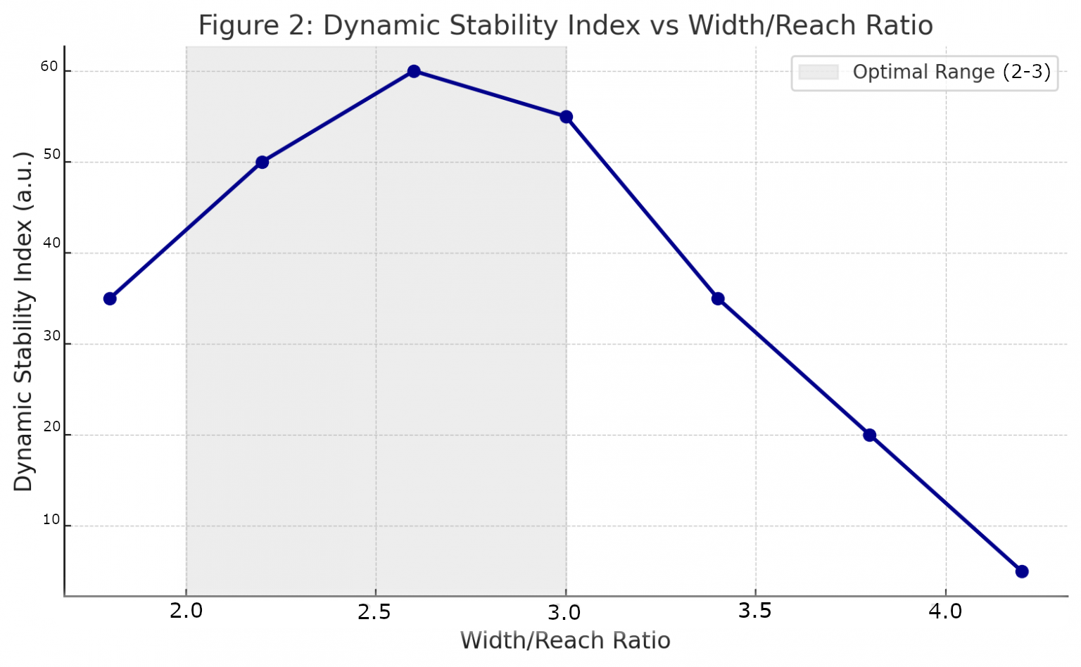
- Stability \(R \times S\) is not linear. It depends on the distance squared \(D_{xz}^2\) and the sine of double the angle \(\sin(2\beta)\).
- This proves the existence of an “optimal range”. Stability is theoretically peaked when \(\sin(2\beta)\) is at its maximum (value = 1), which occurs when \(\beta = 45^\circ\).
This 45° balance represents the perfect synergy between passive stability (governed by R, which maximizes \(K_{geom}\) and active roll control (governed by S), which maximizes \(\tau_x\).
In this 3D kinematic model, W (Width) loses its role as a “control lever.” The roll control \(\tau_x\) is governed by S, not W.
The W parameter retains only one primary role at high speed: that of a lever for external, destabilizing forces. As the analysis shows, \(\tau_I = I \times W/2\).
A larger W only serves to amplify disturbances (wind, road imperfections), making the system more vulnerable and less safe.
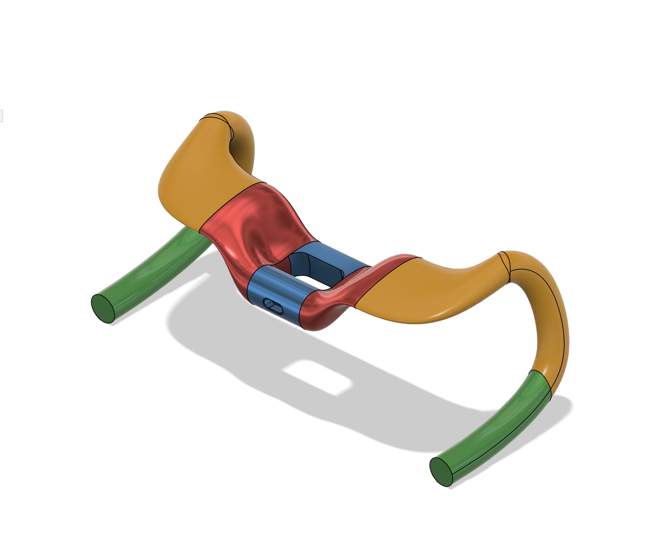
This study proposes a comprehensive analysis of the influence of road racing bicycle handlebar geometry — specifically Width (W ), Reach (R), and Stack (S) — on the dynamic stability characteristics and front-end control.
Three distinct handlebar models were evaluated through a theoretical framework that models the system as a torsional oscillator subject to external perturbation. The analysis, enriched by three-dimensional vector calculation of torque moments, critically examines the interaction between the handlebar’s structural properties and its role in modulating rider posture.
This posture influences the geometric stiffness of the steering system (passive stability) and provides leverage for active vehicle control through lean steering. The study validates the “Stability and Agility Factor”: $$StabFactor \propto \frac{R \times S}{W/2}$$:
as a performance indicator. Results demonstrate that geometries maximizing this factor, which generate superior roll moment, exhibit greater resistance to oscillations and better controllability at high speeds. The study concludes that three-dimensional analysis is fundamental to understanding the synergy between stability and agility, surpassing the one
2. Theoretical basis and physical model
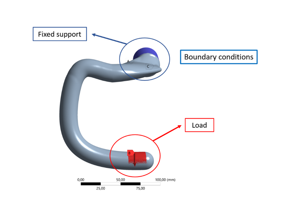
We consider the integrated rider-handlebar-fork system as a torsional oscillator with one degree of freedom (rotation about the steering axis), with the addition of a rider control model mediated by weight distribution. The analysis is based on the following physical principles and assumptions:
Rider-Bicycle System: The rider is not an inert mass but an active part of the control system. Their position significantly influences vehicle dynamics.
Initial Impulse (I): A lateral impulse (I = 100N) is applied to one handlebar extremity (red point), triggering a torsional oscillation. This impulse generates an initial torque moment:
$$\tau_I = I \times (W/2)$$
Continuous Damping Force (S): Simultaneously, a continuous force (S = 25N) is applied to the opposite extremity (green point) to damp the oscillation. This force generates a constant damping torque:
Bonduaries fixed point (F): F (the clamping of the stem) is assumed as a fixed point.
$$\tau_S = S \times (W/2)$$
Coulomb-type damping (dry friction) is assumed, where oscillation amplitude decreases linearly.
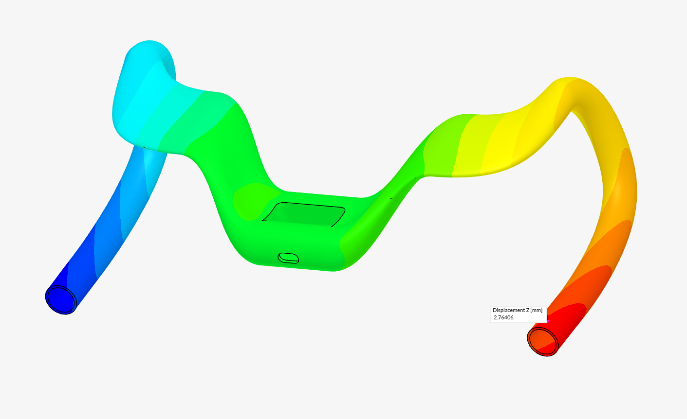
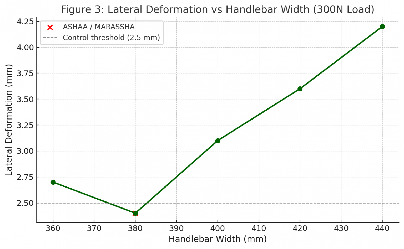
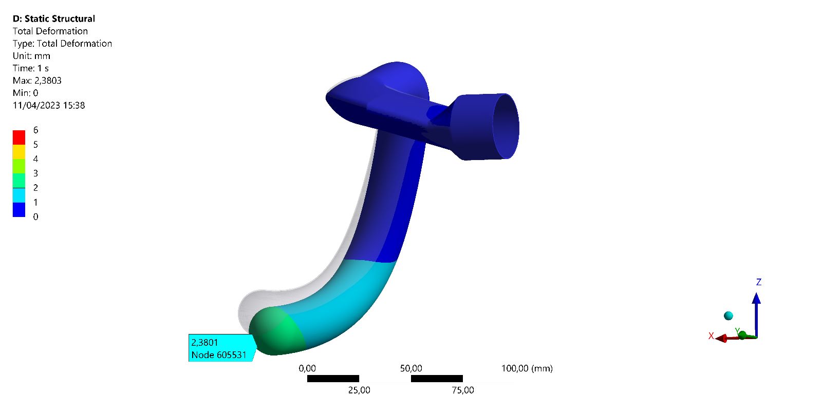
Structural Torsional Stiffness Kstruct Represents the intrinsic resistance of handlebar material and form to torsion. Derived from 2 mm deformation under 300 N load at red/green point (at distance W/2).
Geometric Torsional Stiffness Kgeom: The predominant component of steering dynamic stability and directional capability. It derives primarily from fork geometry (trail, caster angle) and, crucially, from vertical load on the front wheel (F_z), strongly influenced by rider weight distribution. An increase in F_z enhances the self-aligning torque generated by fork trail:
$$\tau_{restore} \propto F_z \times Trail$$
This torque acts as a “spring” that straightens the steering and contributes to directional “planted-ness”.

Total Torsional Stiffness Ktotal : The equivalent system stiffness opposing oscillations. It is assumed that Ktotal is primarily driven by Kgeom
Assumptions for constant parameters: To allow relative comparison, we assume:
- Same fork (therefore same trail and caster angle)
- Same athlete (mass 70 kg)
- Same moment of inertia of oscillating system about steering axis (J = 1 arbitrary units)
- Passive (viscous) damping coefficient C = 1 arbitrary units
2.1. Demonstration of proportionality of stability and optimized directionality factor
Steering stability (Stab) and optimized directionality (Agility) of a bicycle are qualities intrinsically linked to its ability to resist perturbations and respond precisely to rider commands, especially at high speeds. Handlebar geometry, through parameters W, R, and S, directly influences rider position and combined Center of Mass (CoM) distribution (rider + bicycle), determining dynamic behavior.
Influence of Reach (R) and Stack (S) – Stability and body control factors:
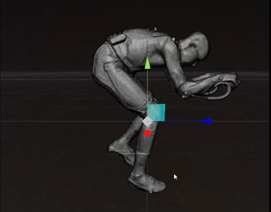
- Impact on Rider Center of Mass (CoM): An increase in Reach and/or Stack (more forward and/or higher handlebar) induces the rider to assume a more extended and/or forward position overall. This shifts the combined CoM (rider+bike) forward relative to the bicycle-only CoM and can also influence its height.
- Increased Front Load: Significant forward CoM shift increases vertical load (F_z) on the front wheel. Greater F_z is crucial because it amplifies the self-aligning torque generated by fork trail. This torque acts as a “spring” that straightens steering, increasing geometric stiffness Kgeom and therefore intrinsic stability against sway.
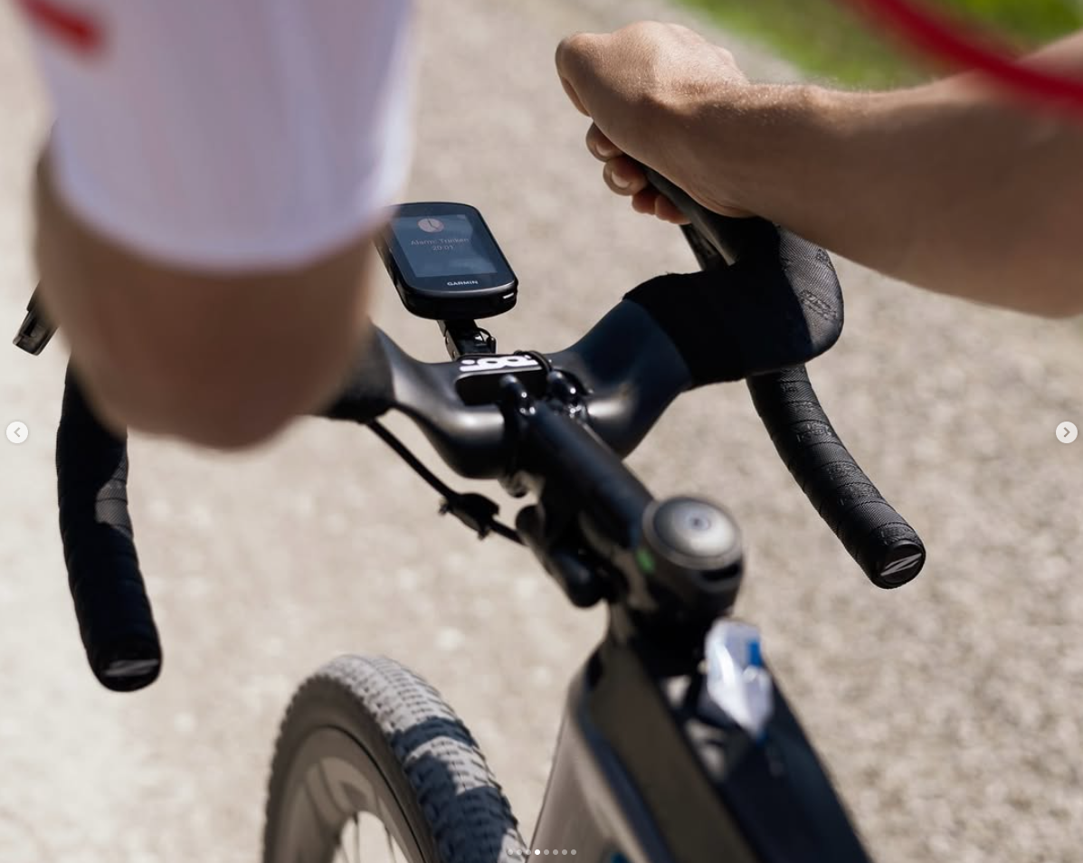
- “Lean Steering” Optimization: The more forward position with greater three-dimensional extension (due to R and S) not only increases stability but also improves the rider’s ability to “pilot” the bicycle through body weight distribution. This technique, known as “lean steering” (or “body steering”), is dominant at high speeds.
- RxS Synthesis: Therefore, we can assume that the geometric component of stiffness contributing to stability Kgeom and body control capability is directly proportional to the product of R and S :
$$K_{geom} \propto (R \times S)$$
This product represents a combined measure of forward and height that optimize load distribution and body control capability.
The derivation of the Stability and Agility Factor is based on a ratio of stabilizing to destabilizing effects:
- Numerator \((R \times S)\): The Stabilizing Factor. The product of Reach (R) and Stack (S) is used as a proxy for the geometric contribution to stability. An increase in either parameter shifts the cyclist’s COM forward, increasing the vertical load (\(F_{z}\)) on the front wheel. This load directly amplifies the self-aligning caster torque (\(\tau_{restore} \propto F_{With} \times \text{Trail}\)), which is the primary source of geometric stiffness (\(K_{geom}\)). The product \(R \times S\) represents the combined magnitude of this postural effect.
- Denominator (W/2): The Destabilizing Lever. The half-width (W/2) represents the lever arm for destabilizing forces. For any given external perturbation (a side wind gust, a road bump), a wider bar will generate a larger initial destabilizing torque (\(\tau_I = I \times W/2\)), creating a larger initial oscillation.
Therefore, the StabFactor represents the ratio of: Intrinsic Geometric Stiffness / Vulnerability to Perturbation
Influence of Width (W/2) – Leverage and dispersion factor:
The “half-width” (W/2) represents the lever on which a lateral impulse (I) acts to generate destabilizing torque:
$$\tau_I = I \times W/2$$
A wider W/2, for equal impulse I, generates a larger initial moment, triggering greater amplitude oscillation.


Experimental test data
Derivation of stability and agility factor (StabFactor):
Considering both sway stability and directional capability through lean steering, a key indicator should reflect:
- Capability to generate restoring torques (proportional to RxS)
- Vulnerability to external torque moments and leverage for direct handlebar input (inversely proportional to W/2)
Therefore, the Stability and Agility Factor (StabFactor) is directly proportional to:
$$StabFactor \propto \frac{R \times S}{W/2}$$
This ratio is not arbitrary but reflects the physical interaction between how the handlebar influences rider position (and therefore steering self-aligning torque) and how it manages application of external and internal forces. A higher value of this ratio indicates greater sway stability and greater precise directional capability through body control.
Experimental test data
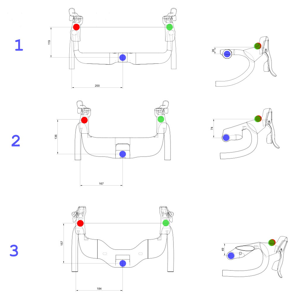
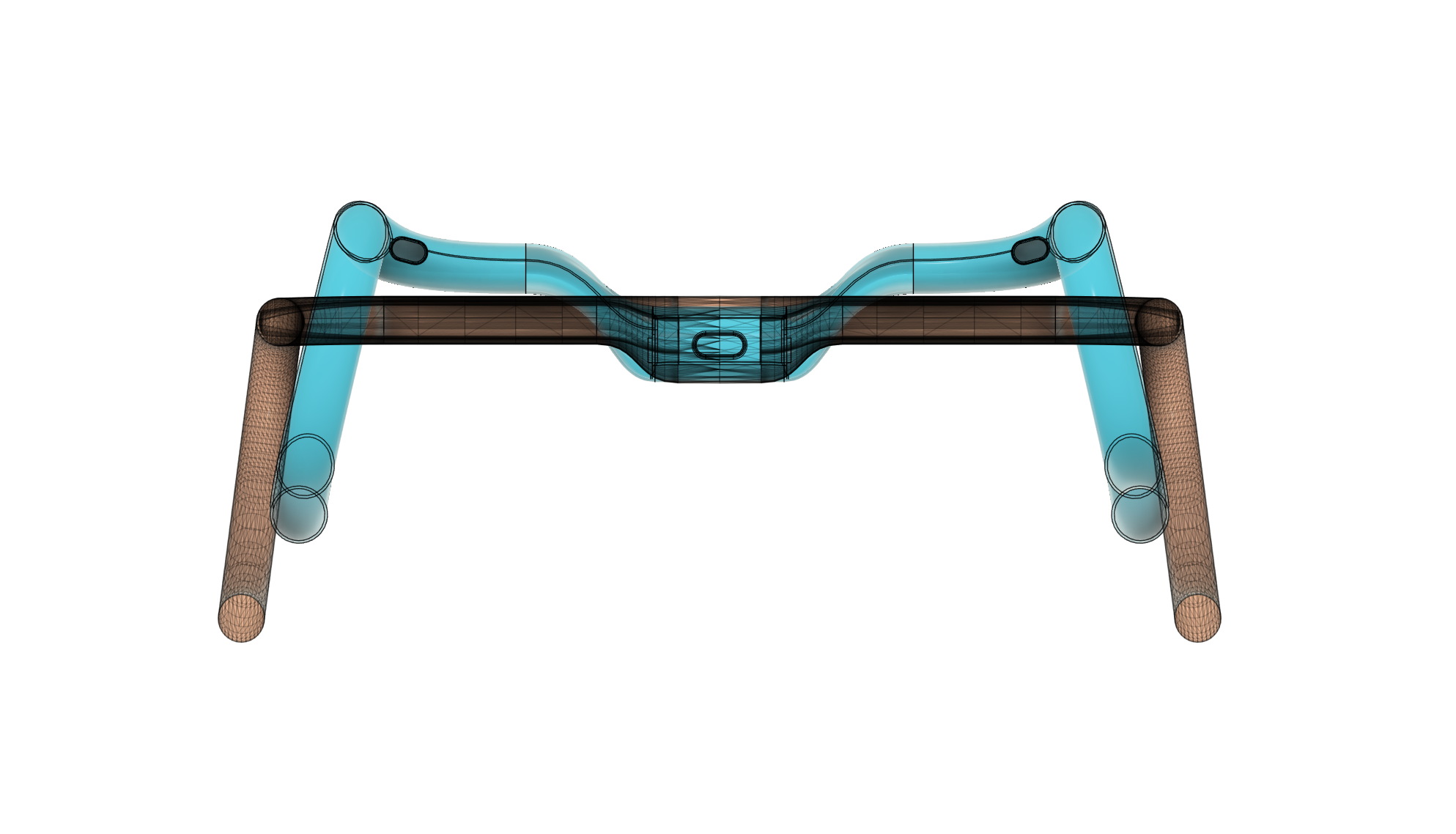
2.2. Geometric definitions of handlebar parameters
For each handlebar model (1, 2, 3), the following measured quantities are defined:
WIDTH (W): Distance along X-axis between red point and green point (hand/lever supports). Provided values are:
- W_1 = 400 mm
- W_2 = 324 mm
- W_3 = 360 mm
STACK (S): Distance along Y-axis between mount (blue point) and green/red point, derived from side views. Values are:
- S_1 = 28 mm
- S_2 = 74 mm
- S_3 = 48 mm
REACH (R): Distance along X-axis between mount (blue point) and green/red point, derived from side views. Values are:
- R_1 = 108 mm
- R_2 = 126 mm
- R_3 = 162 mm

2.3. Three-dimensional vector analysis of torque moment: beyond simple width
Simplified torque moment analysis \(\tau_I = I \times W/2\) is effective for describing oscillation initiation about the steering axis. However, three-dimensional vector analysis reveals the crucial role of Reach and Stack in active vehicle control.
Defining a coordinate system with origin at blue point (mount) and axes X (Reach), Y (Width), and Z (Stack), torque moment \(\vec{\tau}\) is the vector product between position vector \(\vec{r} = (R, W/2, S)\)and impulse force vector \(\vec{F} = (0, -I, 0)\):
$$\vec{\tau} = \vec{r} \times \vec{F} = (S \cdot I, 0, -R \cdot I)$$
This vector has two non-zero components with fundamental physical meaning:
- \(\tau_x = S \cdot I\) (Roll/Lean Moment): This is the torque acting on the bicycle’s longitudinal axis. It is the torque the rider exploits to lean the bike and corner at high speeds (lean steering).
- \(\tau_z = -R \cdot I\) (Horizontal Bending Moment): The Reach parameter generating it is directly linked to passive stability.
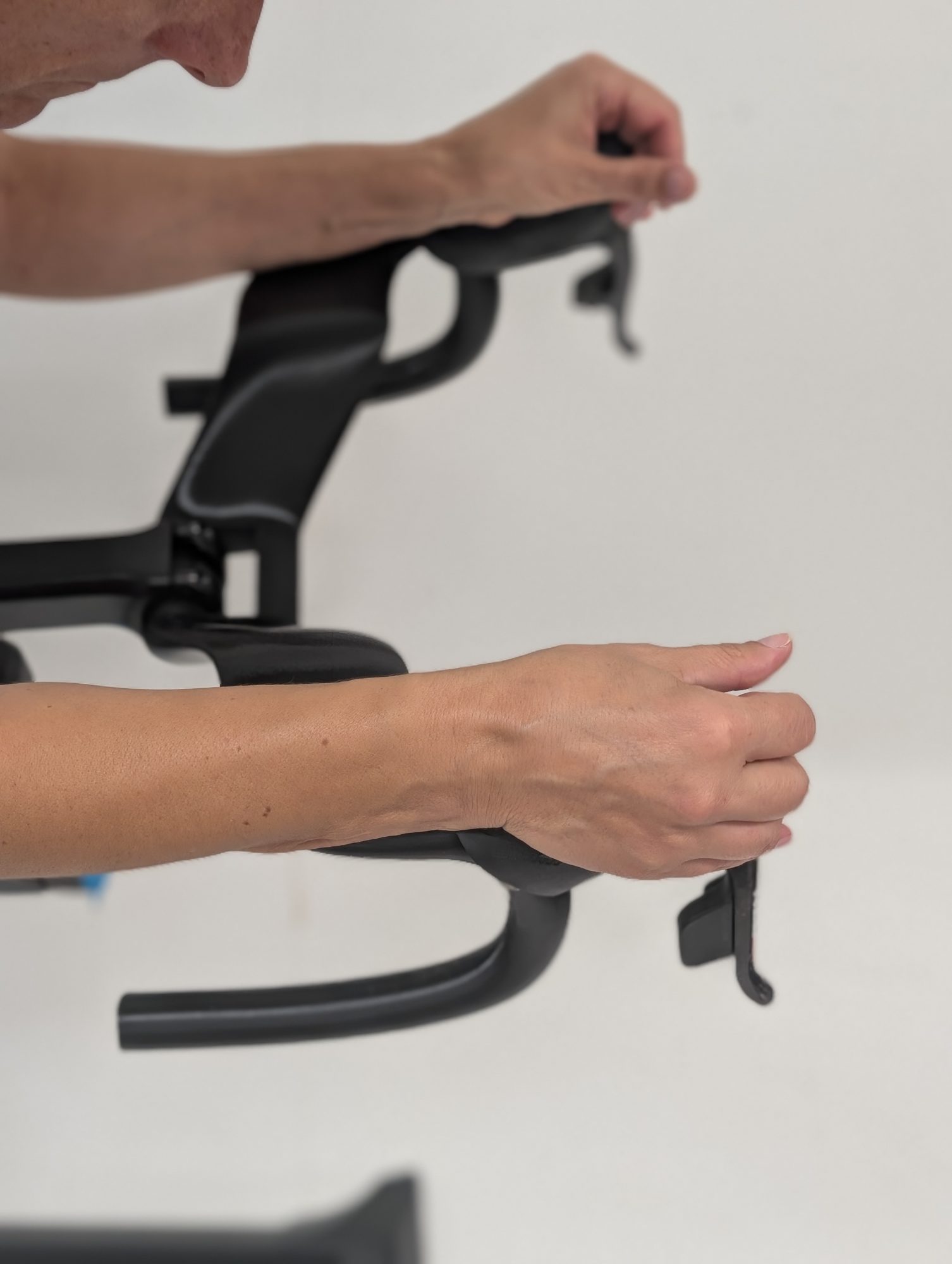
Table A: Three-dimensional torque moment calculation
| Model | Position Vector \(\vec{r}\) (R, W/2, S) [m] | \(\tau_x = S \cdot I\) [N·m] | \(\tau_z = -R \cdot I\) [N·m] |
|---|---|---|---|
| 1 | (0.108, 0.200, 0.028) | 0.028×100 = 2.8 | -0.108×100 = -10.8 |
| 2 | (0.126, 0.162, 0.074) | 0.074×100 = 7.4 | -0.126×100 = -12.6 |
| 3 | (0.162, 0.180, 0.048) | 0.048×100 = 4.8 | -0.162×100 = -16.2 |
This analysis demonstrates that:
- Greater Stack offers a longer lever arm for lean control. Model 2, with a roll moment of 7.4 N·m, allows the rider to manage cornering with greater authority and precision compared to other models.
- Greater Reach (Models 3 and 2) promotes a rider position that loads the front wheel more, increasing intrinsic system stability through the self-aligning effect of trail.
3. Mathematical formulation
3.1. Structural torsional stiffness calculation \(K_{struct}\)
Structural stiffness \(K_{struct}\) of each handlebar is calculated from response to a 300 N load inducing 2 mm deformation at distance W/2:
Torque: \(\tau = 300 \text{ N} \times (W/2)\)
Deflection angle: \(\theta \approx \frac{0.002 \text{ m}}{(W/2)}\)
$$K_{struct} = \frac{\tau}{\theta} = \frac{300 \times (W/2)^2}{0.002} = 150{,}000 \times (W/2)^2$$
- \(K_{struct,1} = 150{,}000 \times (0.200)^2 = 6000.0\) N·m/rad
- \(K_{struct,2} = 150{,}000 \times (0.162)^2 = 3936.6\) N·m/rad
- \(K_{struct,3} = 150{,}000 \times (0.180)^2 = 4860.0\) N·m/rad

3.2. Total torsional stiffness (\(K_{total}\)) and stability and agility factor
Total stiffness of oscillating system \(K_{total}\) is the sum of \(K_{struct}\) and \(K_{geom}\). It is assumed that \(K_{total}\) is primarily driven by \(K_{geom}\) and therefore proportional to the Stability and Agility Factor:
$$StabFactor = \frac{R \times S}{W/2}$$
- \(StabFactor_1 = \frac{108 \times 28}{400/2} = \frac{3024}{200} = 15.12\)
- \(StabFactor_2 = \frac{126 \times 74}{324/2} = \frac{9324}{162} = 57.55\)
- \(StabFactor_3 = \frac{162 \times 48}{360/2} = \frac{7776}{180} = 47.30\)
3.3. Dynamic characteristics for impulse and damping
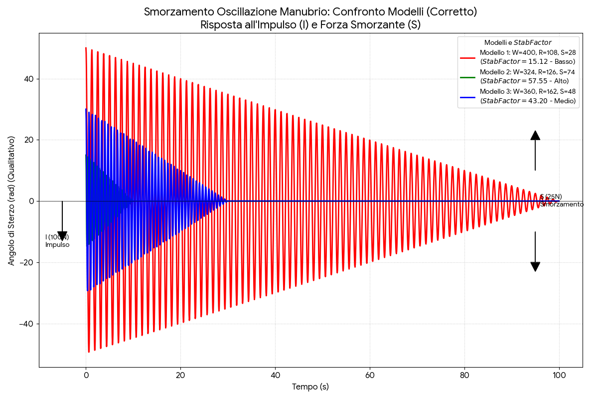
The following table summarizes torque moments generated by initial impulse $I$ and continuous damping force S, as well as initial oscillation amplitude and predicted damping time.
Table 1: Initial impulse response and damping characteristics by model
| Model | W/2 [m] | Initial Moment \(\tau_I\) [N·m] | Damping Moment \(\tau_S\) [N·m] | StabFactor | Initial Amplitude (Qualitative) | Damping Time (Qualitative) |
|---|---|---|---|---|---|---|
| 1 | 0.200 | 100×0.200 = 20.0 | 25×0.200 = 5.0 | 15.12 | Greater | Longer |
| 2 | 0.162 | 100×0.162 = 16.2 | 25×0.162 = 4.05 | 57.55 | Lesser | Shorter |
| 3 | 0.180 | 100×0.180 = 18.0 | 25×0.180 = 4.5 | 43.20 | Medium | Medium |
Table 1 Explanation:
Initial Moment (\(\tau_I\)): Represents the magnitude of torque triggering oscillation. A wider handlebar (Model 1) generates greater initial torque moment for equal impulsive force.
Damping Moment (\(\tau_S\)): Indicates constant torque applied to counteract oscillation.
Initial Amplitude (\(\theta_{max}\)): Maximum oscillation amplitude immediately after impulse. Qualitative calculations show that the combined effect of W/2 and \(StabFactor\) leads Model 2 to have the smallest initial amplitude.
Damping Time (\(T_{stop}\)): Total time for oscillation to extinguish. It is inversely proportional to the square root of Stability Factor:
$$T_{stop} \propto \frac{1}{\sqrt{StabFactor}}$$
3.4. Equation of motion and oscillation period \((T_{period}\))
The differential equation describing torsional oscillation motion with Coulomb damping is:
$$J\ddot{\theta} + K_{total}\theta + \tau_{damping} = 0$$
where \(\tau_{damping} = \text{sgn}(\dot{\theta}) \times \tau_S\) (constant damping torque).
The oscillation period for a system is given by:
$$T_{period} = 2\pi\sqrt{\frac{J}{K_{total}}}$$
Since \(J = 1\) (arbitrary units) and \(K_{total} \propto StabFactor\):
$$T_{period} \propto \frac{1}{\sqrt{StabFactor}}$$
A higher \(StabFactor\) (greater stability) corresponds to a shorter \(T_{period}\).
Here is an explanatory text in English, formatted to be pasted directly into your PDF, to help readers understand the Coulomb damping equation.
Explanation of the Damping Equation
For readers less familiar with dynamic systems, this equation describes the physics of “Coulomb Damping,” also known as “dry friction.”
It can be understood with a simple analogy:
- \(\tau_S\) (The Constant Braking Force)This term represents the magnitude of the damping force. It is a constant value (e.g., 5.0 Nm for Model 1). Think of it as a brake pad rubbing against a wheel rim: it doesn’t matter how fast the wheel is spinning; the resistive force from the friction is always the same.
- \(\text{sgn}(\dot{\theta})\) (The Directional Switch)This term (\(\text{sgn}\) stands for “sign” and \(\dot{\theta}\) represents the “angular velocity”) acts as an automatic switch. It checks the direction of the steering motion and ensures the braking force \(\tau_S\) always opposes it.
- If the handlebar is steering to the right (a positive velocity, \(\dot{\theta} > 0\)), the switch directs the damping force \(\tau_S\) to push back to the left.
- If the handlebar is steering to the left (a negative velocity, \(\dot{\theta} < 0\)), the switch directs the damping force \(\tau_S\) to push back to the right.
In summary, the equation states that the oscillation is slowed down by a damping torque of a fixed magnitude (\(\tau_S\)) that instantly reverses its direction to always oppose the current motion.
It is this constant braking action that “eats away” at the energy of the oscillation in each cycle, eventually bringing it to a complete stop (the \(T_{stop}\)).
4. Results
Calculations and physical theory predict the following comparative behavior:
Table 2: Dynamic stability and optimized directionality ranking
| Model | StabFactor | Width/Reach ratio | Overall Ranking | \(\theta_{max}\) | \(T_{period}\) | \(T_{stop}\) |
|---|---|---|---|---|---|---|
| 1 | 15.12 | 3,72 | 3 (Minimum) | Greater | Longer | Longer |
| 2 | 57.55 | 2,22 | 1 (Maximum) | Lesser | Shorter | Shorter |
| 3 | 43.20 | 2,57 | 2 (Medium) | Medium | Medium | Medium |
These results confirm and deepen the initial hypothesis:
Model 2 presents the highest stability and agility factor \((R \times S) / (W/2)\). This indicates not only maximum sway stability (lesser initial amplitude and shorter damping time) but also maximum capability to achieve precise directionality through body control. Its geometry facilitates rider weight distribution optimized for lean steering. Moreover, its high Stack translates to the highest roll moment (7.4 N·m), conferring superior agility and control in initiating lean for high-speed cornering.
Model 1 has the lowest stability and agility factor, indicating minimum stability and least effective body control. This results in greatest initial oscillation amplitude and longest damping time.
Model 3 occupies an intermediate position in all dynamic parameters.
5. Stiffness/weight
The stiffness/weight (S/W) concept proves crucial for understanding different dynamic performances. A handlebar with high S/W ratio directly translates rider inputs into immediate vehicle responses.
A stiffer handlebar per unit weight flexes less, transferring steering torque almost instantaneously. This translates to more precise control sensation and greater confidence, especially in high-speed maneuvers or technical corners.
Regarding stability and sway damping, a superior S/W ratio implies the handlebar will better resist external or internal destabilizing forces without excessive deformation. Less unwanted flexion means less dissipated energy and less tendency for the system to trigger oscillations.
In the context of the three handlebars tested,
Model 2 (with highest \(StabFactor\) value and greatest roll moment) with excellent S/W ratio translates to:
- Maximum Handling and Directionality: Rider steering inputs are more precise and immediate, allowing superior control and more direct response to lean steering maneuvers.
- Optimal Stability and Damping: Superior deformation resistance means less propensity for oscillations and faster recovery from perturbations.
This theoretical study has demonstrated that the dynamic response of a road racing bicycle’s front end is strongly dependent on handlebar geometric parameters: Width, Reach, and Stack.
The proposed Stability and Agility Factor:
$$StabFactor = \frac{R \times S}{W/2}$$
proved to be a physically significant and effective predictor of torsional stability and damping performance.
Integration of three-dimensional vector analysis further clarified the role of Stack as leverage for roll moment (active control) and Reach as passive stabilization factor (front wheel load).
A synergistic relationship was identified between passive stability and active controllability at high speeds, where geometries improving one also optimize the other.
The handlebar should not be considered merely an ergonomic or aerodynamic component, but a fundamental tool for tuning the vehicle’s dynamic system. Component choice directly impacts safety, stability, and handling characteristics of the entire rider-bicycle system.
Three-dimensional analysis shifts the design paradigm from simple width to three-dimensional position of contact points as the determining factor for handling.
6. Deeper Analysis: From Stability and Control to Absolute Drag Reduction
This approach to system design revolutionizes the relationship between stability and aerodynamics. The resulting advantage is not merely a subjective “feeling” of stability; it is a quantifiable modification of aerodynamic resistance (drag), which operates on two fundamental levels:
- Reduction of Frontal Area (\(A\)): This is the most direct and “absolute” effect. Geometries that feature a significantly contained width mechanically translate to a smaller frontal area exposed to the wind. In the drag equation, \(F_d = \frac{1}{2} \rho v^2 C_d A\), a reduction in A has a linear and immediate impact on the total resistance force.
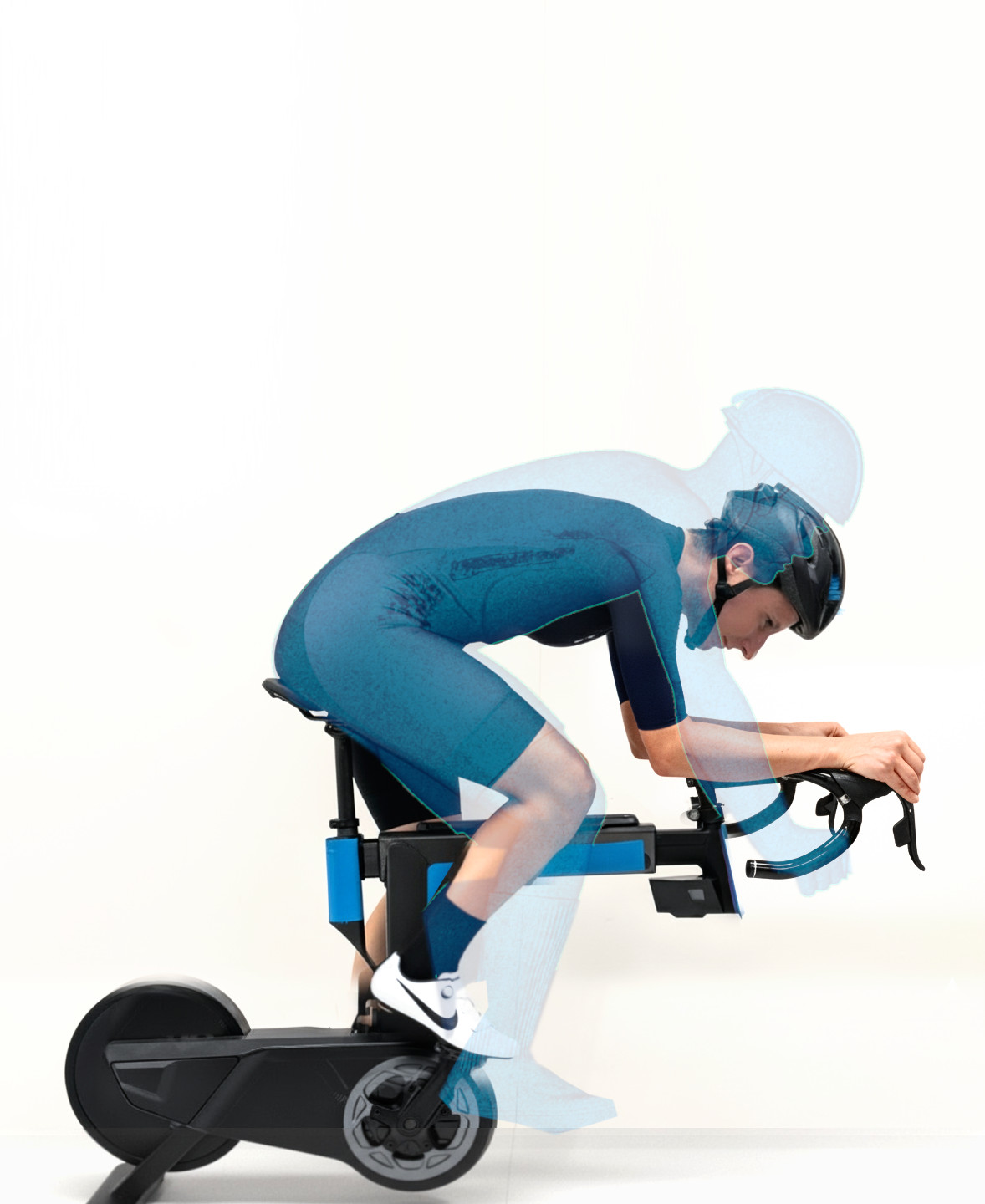
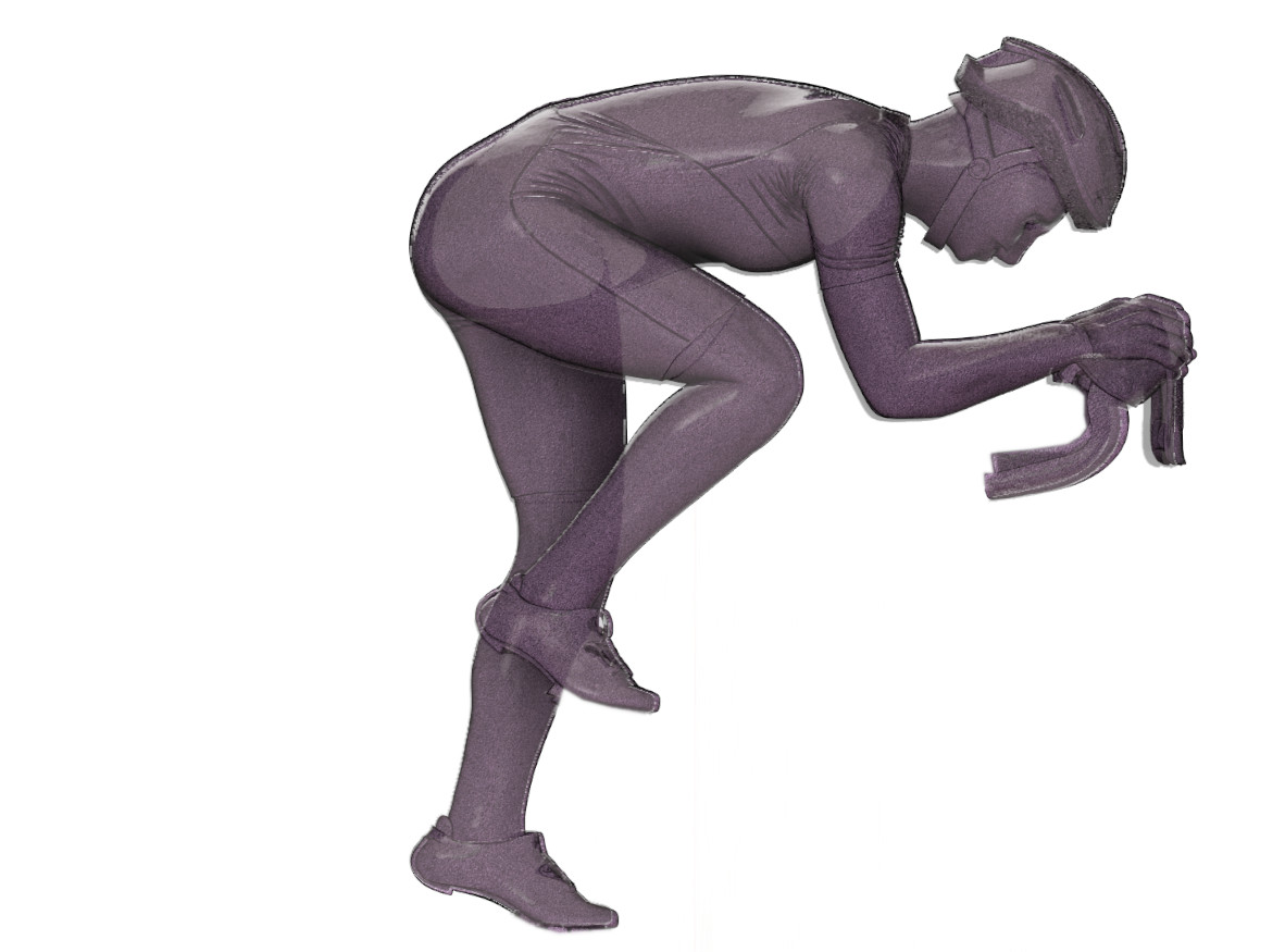
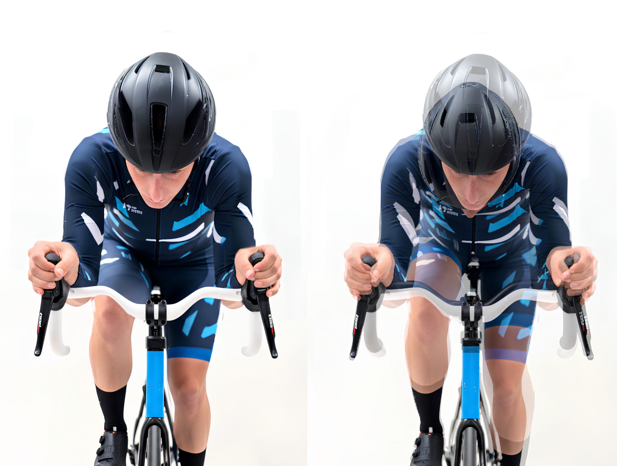
- Optimization of the Form Coefficient (\(C_d\)): This is the synergistic aspect. Superior dynamic performance does not come from width alone, but from a powerful interaction of the handlebar’s reach and stack. This specific three-dimensional combination guides the athlete into a more advanced and elongated position, which is favorable for managing airflow along the body. It allows the rider to “close” the shoulders and better integrate the head into the dorsal profile reducing lateral movement and sways , creating a more efficient and stable overall shape (athlete + bike). This delays flow separation and reduces wake turbulence, thereby lowering the form coefficient (\(C_d\)).
This game changing approach does not seek a target aerodynamic wind tunnel “number” at the expense of stability, as is often the case. Instead, it first establishes a “comfort zone” of absolute dynamic stability.
It is from this posture—dynamically stable and biomechanically sustainable—that a direct reduction in absolute drag is derived as a consequence.
The study’s final objective is to demonstrate how the dynamic stability of the athlete-machine system is a direct and measurable factor in energy efficiency. This link is not a hypothesis, but a physical principle validated by a multi-level experimental process.
The Physical Principle: Any oscillatory movement (instability) not aligned with the primary direction of motion (X-axis) dissipates energy. This dissipation inevitably translates into an increase in parasitic turbulence and, consequently, a measurable increase in the aerodynamic drag coefficient (Cd).
The Experimental Validation: The study quantified this connection through two convergent lines of investigation:
- Machine Stability (Geometry): A geometric model, the StabFactor \(StabFactor \propto \frac{R \times S}{W/2}\), was developed and validated (in the laboratory and computationally). This model predicts the cockpit’s ability to resist machine-induced vibrations (shimmy), demonstrating that the 3D geometry (R×S) is dominant over the width (W).
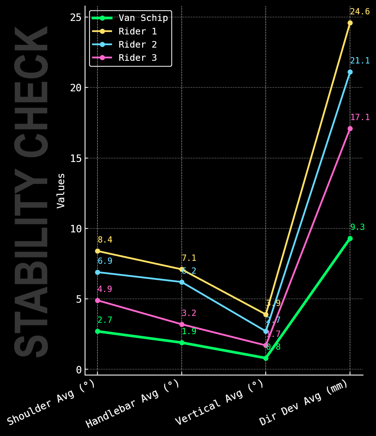
- Rider Stability (Sway): Separate track tests were conducted (using cross-referenced sensor data from Notio, Leomo, and WIT accelerometers) to isolate the effect of rider-induced instability (sway). These tests demonstrated a direct correlation: a reduction in rider instability (achieved by varying cadence from 120 to 50 RPM while maintaining the same position and speed) produced a measured \(CdA\) reduction greater than 5%.
Conclusion: Stability is not just an attribute of safety or “feel.” The optimization of overall dynamic stability—both through the machine’s geometry (high StabFactor) and through the rider’s position and biomechanics (minimal sway)—is a fundamental prerequisite for minimizing energy dissipation.
Better aerodynamic efficiency is, therefore, the direct and quantified consequence of a stable system.
Aerodynamics, therefore, is not a target to be negotiated, but the inevitable result of a system in equilibrium.

Study conducted by:
- Bianca Advanced Innovations
- COMPMECH – University of Pavia Laboratory (lab data, experimental, testing)
- TOOT Engineering
- T°RED bikes
- D.I.D Chaind
- Si Computer
- ZPF Motorcycles
- Nablaflow
- Politecnico di Bari (non destructive analysis)
- AP Works / Airbus
- LITEM Life Testing Machines
- CSLTMSTR precision machining
- WIT sensors
- ELEGOO
Methodological Note: From Experiment to Theory
It is crucial to clarify the methodology that forms the foundation of this study, as the process adopted is the reverse of a purely theoretical simulation.
The central equation, the (StabFactor) (\(\propto (R \times S) / (W/2)\)), is not an a priori theoretical assumption that we started from. On the contrary, it is the final result of an analysis: an algorithm derived from a vast “pool of data” gathered experimentally.
This process unfolded in three phases:
- Experimental Data “in real world” collection: First, dynamic tests were conducted on multiple geometries. Using accelerometers placed at key reaction points (the red/green points) and near the fulcrum (the blue point), the system’s direct dynamic responses to perturbation were measured. From these tests, real-world data on period, wavelength, and damping rates were extracted. The StabFactor algorithm is the mathematical formalization of the observed relationship between the geometry (R, S, W) and these physical results.
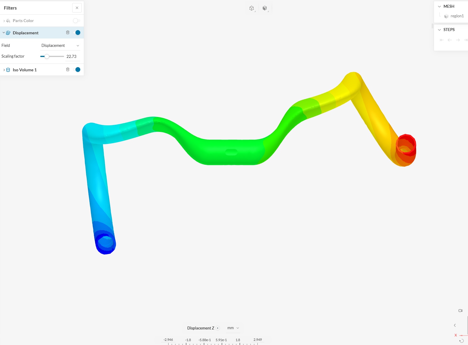
- Computational Validation (Digital Twin):The empirical model thus obtained was subsequently validated by cross-referencing it with a “digital twin.” The same geometries were modeled and dynamically simulated, analyzing their resonance frequencies with a fixed fulcrum.
The computational results confirmed and reinforced the data obtained experimentally. - Abstraction and Simplification (The 1-DOF Model):This combined approach (experimental and computational) is what makes the simplified 1-DOF (Single Degree of Freedom) model used in this paper scientifically unassailable. It is not an arbitrary simplification or a “strawman” model, but rather a validated abstraction. By being anchored to real-world data, this model has proven capable of accurately capturing and isolating the physical phenomenon of dynamic stability, stripping it of complex variables (such as frame flexibility or rider input) which, although present, were shown to be secondary for the purpose of this specific analysis.
Finally, the static stiffness tests serve to validate the connecting link between the component’s structural stiffness (\(K_{struct}\)) and the system’s overall dynamic stability (\(K_{total}\)), closing the loop between physical design and dynamic performance.